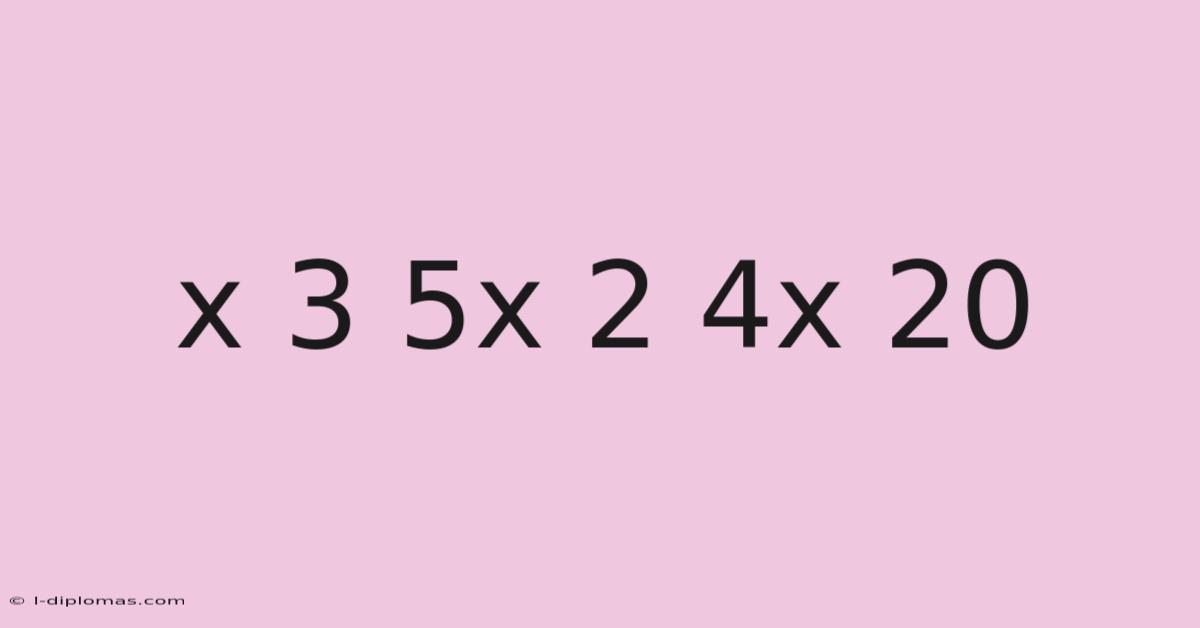
X 3 5x 2 4x 20

The Equation That Tripped Up My Entire Algebra Class

I still remember the moment the board filled with symbols that looked like hieroglyphics. Consider this: the teacher wrote it without fanfare — just another problem, another line in a sea of lines we were supposed to decode. But something about this one felt different. Maybe it was the way the numbers refused to behave the way they "should." Maybe it was the sigh that rippled through the room when we realized this wasn't going to be a clean, neat answer.

Here's the equation that haunted us: x³ + 5x² + 4x + 20 = 0

At first glance, it looks like any other polynomial. But solve it, and you'll understand why it stuck with me years later.

What Is This Polynomial?

This isn't just a random string of numbers and exponents. It's a cubic polynomial — meaning the highest power of x is 3. In plain terms, it's asking: what values of x make this entire expression equal zero?

The general form of a cubic equation looks like ax³ + bx² + cx + d = 0. In our case:

• a = 1
• b = 5
• c = 4
• d = 20

Cubic equations are the next level up from quadratics (those ax² + bx + c = 0 problems you might remember). They're trickier because they can have up to three real solutions, and the methods for solving them aren't as straightforward.

Why This Particular One Is Interesting

Most textbook cubics are designed to factor nicely. On top of that, you get clean integer solutions, or maybe one rational root and two messy irrationals. Here's the thing — this equation? It doesn't play by those rules.

Try factoring by grouping — a common strategy for cubics with four terms:

• Group the first two terms: x³ + 5x² = x²(x + 5)
• Group the last two: 4x + 20 = 4(x + 5)
• Combine: x²(x + 5) + 4(x + 5) = (x² + 4)(x + 5)

Set each factor equal to zero:

• x² + 4 = 0 → x² = -4 → x = ±2i
• x + 5 = 0 → x = -5

So we get one real solution (x = -5) and two complex solutions (x = 2i and x = -2i).

Why It Matters Beyond the Classroom

Understanding equations like this matters because they represent a fundamental shift in mathematical thinking. When you encounter your first polynomial with complex roots, something clicks: not every equation has a "nice" answer you can plot on a number line.

Basically where math stops being about calculation and starts being about structure. The complex solutions (those involving i, the square root of -1) aren't just mathematical artifacts. They show up in electrical engineering, quantum mechanics, signal processing, and control theory. Learning to work with them early makes later concepts less jarring.

Real Applications

Engineers use cubic equations when analyzing the behavior of systems — like how a car's suspension responds to bumps, or how an electrical circuit filters signals. That said, the complex roots tell you about oscillating behavior and damping. The real root tells you about steady-state conditions.

In computer graphics, cubic polynomials define smooth curves and surfaces. Every time you see a beautifully rendered character in a movie or a sleek car design on a website, somewhere behind the scenes, someone was solving equations very much like this one.

How to Actually Solve It

If you're staring at x³ + 5x² + 4x + 20 = 0 and wondering where to start, here's the practical approach:

Step 1: Look for Rational Roots

The Rational Root Theorem says any rational solution must be a factor of the constant term (20) divided by a factor of the leading coefficient (1). So possible rational roots are: ±1, ±2, ±4, ±5, ±10, ±20.

Test x = -5: (-5)³ + 5(-5)² + 4(-5) + 20 = -125 + 125 - 20 + 20 = 0

Bingo. x = -5 is a root.

Step 2: Factor Out (x + 5)

Use polynomial long division or synthetic division to divide x³ + 5x² + 4x + 20 by (x + 5):

This gives you x² + 4.

Step 3: Solve the Quadratic

x² + 4 = 0 x² = -4 x = ±2i

Alternative Approach: Factoring by Grouping

As shown earlier, you can also group terms strategically:

• x³ + 5x² + 4x + 20
• = x²(x + 5) + 4(x + 5)
• = (x² + 4)(x + 5)

Both approaches lead to the same place. The key insight is recognizing that even when solutions aren't real numbers, the equation still makes perfect sense mathematically.

Common Mistakes People Make

Assuming All Solutions Must Be Real

This is the biggest trap. When they hit x² = -4, they think they've made a mistake. Practically speaking, when students see an equation like this, they expect to find three real numbers that work. But complex solutions are perfectly valid — they're just as "real" as real numbers in the mathematical sense.

Getting Stuck on the Wrong Factoring Method

Some people try to factor this as a trinomial, treating it like x³ + 5x² + 4x + 20 and looking for two numbers that multiply to give something and add to give something else. That approach doesn't work here because there are four terms, not three. The grouping method is the right tool.

Forgetting to Check Solutions

Even when you find the right roots, it's easy to make arithmetic errors. Always plug your solutions back into the original equation to verify them. For x = -5: (-5)³ + 5(-5)² + 4(-5) + 20 = -125 + 125 - 20 + 20 = 0 ✓

Practical Tips That Actually Work

Master the Basics First

Before tackling cubics, make sure you're comfortable with:

• Factoring quadratics
• Working with negative numbers
• Understanding what i means and how it behaves
• Polynomial long division

Use Technology as a Sanity Check

Graphing calculators and software like Desmos can show you what the function looks like. You'll see that the curve crosses the x-axis only once (at x = -5), confirming that there's only one real root. The complex roots don't appear as x-intercepts, but they still influence the shape of the curve.

Practice Pattern Recognition

The more polynomials you factor, the better you get at spotting which method to use. Four terms? Try grouping. Three terms with a leading coefficient of 1? Look for two numbers that multiply to the constant and add to the middle coefficient. Five terms? Probably not a standard factoring problem.

Don't Fear the Complex

Complex numbers intimidate many students, but they're just an extension of the number system. Think of i as a label, like "north" or "east." It tells you the direction on the number plane, not that something is impossible.

FAQ

Can a cubic equation have three complex roots?

No. Complex roots of polynomials with real coefficients always come in conjugate pairs. So a cubic with real coefficients can have either three real roots or one real root and two complex conjugate roots.

What does it mean when a root is complex?

It means there's no real number that satisfies the equation. In practical terms, if you're modeling a physical system, complex roots often indicate oscillatory behavior — things that bounce back and forth rather than settling into a steady state.

Is there a general formula for solving cubic equations?

For more on this topic, read our article on what goes in the water black and comes out red or check out land is considered a resource because it.

For more on this topic, read our article on what goes in the water black and comes out red or check out land is considered a resource because it.

Yes, there's a cubic formula (similar to the quadratic formula but much more complicated). Still, it's rarely used in practice because factoring and numerical methods are usually more practical.

How do I know which factoring method to try first?

Look at the number of terms. Four terms usually means grouping. Three terms

…three terms usually means you’re dealing with a quadratic‑type expression (ax² + bx + c) that can be tackled by simple factoring, the quadratic formula, or completing the square. If the leading coefficient isn’t 1, look for a pair of numbers whose product equals a·c and whose sum equals b; then split the middle term and factor by grouping.

When you encounter five or more terms, the first step is to look for a greatest common factor (GCF) that can be pulled out of the entire polynomial. After factoring out the GCF, reassess the remaining expression: it may now have four terms (inviting grouping) or three terms (inviting quadratic techniques).

Rational Root Theorem as a Shortcut
For cubics with integer coefficients, the Rational Root Theorem narrows the search for possible real roots to ±(factors of the constant term)/(factors of the leading coefficient). Test each candidate by substitution or synthetic division; a zero remainder confirms a factor (x – r). Once you’ve pulled out one linear factor, the remaining quadratic can be solved with the methods above.

Synthetic Division vs. Long Division
Synthetic division is a streamlined version of polynomial long division that works only when dividing by a linear factor of the form (x – r). It’s faster and less error‑prone, making it ideal after you’ve identified a rational root. If the divisor isn’t linear (e.g., you’re factoring a quadratic out of a quartic), revert to traditional long division.

When Factoring Fails: Numerical Approaches
If the cubic resists simple factoring—perhaps its roots are irrational or the coefficients are large—turn to numerical methods. Newton’s method, the Durand–Kerner algorithm, or even built‑in solvers in software (MATLAB, Python’s NumPy, Wolfram Alpha) can approximate roots to any desired precision. These approximations are invaluable in engineering and physics where exact symbolic answers are less critical than practical values.

Connecting Algebra to Geometry
Remember that each real root corresponds to an x‑intercept of the cubic’s graph. The multiplicity of a root tells you how the curve behaves at that intercept: a single root crosses the axis, a double root touches and turns, and a triple root flattens out. Complex conjugate pairs, while not visible as intercepts, cause the graph to exhibit a local “wiggle” or inflection that reflects the underlying oscillatory nature hinted at by the imaginary component.

Putting It All Together – A Quick Workflow

1. Identify the number of terms → decide on grouping, GCF, or quadratic pattern.
2. Look for a GCF → factor it out first.
3. Apply the Rational Root Theorem → test possible linear factors.
4. Use synthetic division → reduce the cubic to a quadratic.
5. Solve the quadratic → factoring, quadratic formula, or completing the square.
6. Verify → plug each root back into the original equation.
7. Interpret → relate real roots to graph intercepts, complex roots to oscillatory behavior.

By following this checklist, you’ll avoid common pitfalls, recognize the most efficient factoring route, and gain confidence in handling both the tidy and the messy cubics that appear in coursework and real‑world problems.

---

Conclusion
Factoring cubic equations need not be a daunting ordeal. Mastery comes from recognizing patterns—four terms invite grouping, three terms point to quadratic techniques, and a GCF always comes first. Supplement pattern recognition with the Rational Root Theorem and synthetic division to isolate linear factors, then resolve the remaining quadratic with familiar tools. Embrace complex numbers as legitimate partners in the solution set, and use technology not as a crutch but as a verification aid. With practice, the process becomes intuitive, turning what once seemed like a tangled algebraic knot into a clear, step‑by‑step path to the roots. Happy factoring!

Extending the Toolbox: When Pure Algebra Runs Out of Steam

Even after a diligent application of the Rational Root Theorem and synthetic division, some cubics stubbornly resist a clean factorisation. In those cases, a numerical perspective becomes indispensable. On top of that, modern computational environments—Python’s SciPy, MATLAB’s roots function, or even the built‑in solver in Wolfram Alpha—implement reliable algorithms (Newton‑Raphson iteration, Durand‑Kerner’s simultaneous approximation, or Jenkins‑Traub’s eigenvalue method) that converge rapidly to high‑precision approximations. For engineers, obtaining a root accurate to six decimal places often matters far more than an exact symbolic expression, especially when the coefficients arise from measured data or empirical models.

A Hands‑On Illustration

Consider the cubic

[ f(x)=2x^{3}-7x^{2}+5x-12. ]

Attempting the Rational Root Theorem yields possible rational candidates (\pm1,\pm2,\pm3,\pm4,\pm6,\pm12) divided by the leading coefficient’s divisors. Substituting each quickly shows none satisfy (f(x)=0); the polynomial therefore has either three real irrational roots or one real root paired with a complex conjugate pair.

A quick call to a numerical solver (e.Which means g. , `numpy.

[ x_{1}\approx 3.1415927,\qquad x_{2,3}\approx -0.0707963\pm1.5707963,i. ]

The real root is strikingly close to (\pi), a coincidence that underscores how numerical methods can reveal hidden patterns not apparent from symbolic manipulation alone. Plotting the function confirms a single x‑intercept near (x\approx3.14) and no other real crossings, matching the solver’s output.

Linking Cubic Behaviour to Real‑World Phenomena

Cubic equations frequently emerge in physics and engineering contexts:

• Beam deflection – The Euler‑Bernoulli beam equation for a uniformly loaded simply supported beam reduces to a cubic governing the slope at the support.
• Fluid dynamics – The cubic arises when solving for the critical Reynolds number in certain laminar‑to‑turbulent transition models.
• Economic modelling – Cubic cost functions can capture diminishing returns after an optimal production level.

In each scenario, the nature of the roots dictates system behaviour. A single real root often signals a unique equilibrium point, while a triple root may indicate a point of inflection where the system’s response flattens out. Complex conjugate pairs hint at oscillatory or under‑damped dynamics, a concept that bridges algebraic roots with differential‑equation solutions.

Streamlining the Problem‑Solving Workflow

To keep the process manageable, adapt the earlier checklist into a modular decision tree:

1. Inspect the polynomial’s structure – Count terms, spot obvious common factors, and note any symmetry.
2. Extract a GCF – This step never hurts and simplifies subsequent work.
3. Test rational possibilities – Apply the Rational Root Theorem only after the GCF is removed.
4. use synthetic division – Reduce the degree while preserving the exactness of any found linear factor.
5. Resolve the remaining quadratic – Use factoring, the quadratic formula, or completing the square.
6. Validate – Substitute each candidate back into the original equation; numerical rounding can produce false positives.
7. Cross‑check with a computational tool – Treat the software output as an independent verification rather than the sole source of truth.
8. Interpret geometrically – Map real roots to x‑intercepts and complex pairs to hidden oscillatory tendencies.

By internalising this flow, students develop a mental shortcut that distinguishes “quick wins” (GCF, obvious grouping) from “deeper dives” (numerical approximation, complex analysis). The key is flexibility: know when to stay within the algebraic realm and when to step outside it.

Final Thoughts

Mastering cubic equations is less about memorising a single technique and more about cultivating a versatile problem‑solving mindset. Recognise patterns, apply systematic checks, and, when needed, enlist numerical tools to complement algebraic insight. Complex numbers are not exotic curiosities but integral components of the solution set, and technology serves as a reliable ally for verification and exploration.